 Network congestion may occur when a sender overflows the network with too many packets. At the time of congestion, the network cannot handle this traffic properly, which results in a degraded quality of service (QoS). The typical symptoms of a congestion are: excessive packet delay, packet loss and retransmission.
Insufficient link bandwidth, legacy network devices, greedy network applications or poorly designed or configured network infrastructure are among the common causes of congestion. For instance, a large number of hosts in a LAN can cause a broadcast storm, which in its turn saturates the network and increases the CPU load of hosts. On the Internet, traffic may be routed via the shortest but not the optimal AS_PATH, with the bandwidth of links not being taken into account. Legacy or outdated network device may represent a bottleneck for packets, increasing the time that the packets spend waiting in buffer. Greedy network applications or services, such as file sharing, video streaming using UDP, etc., lacking TCP flow or congestion control mechanisms can significantly contribute to congestion as well.
The function of TCP (Transmission Control Protocol) is to control the transfer of data so that it is reliable. The main TCP features are connection management, reliability, flow control and congestion control. Connection management includes connection initialization (a 3-way handshake) and its termination. The source and destination TCP ports are used for creating multiple virtual connections. A reliable P2P transfer between hosts is achieved with the sequence numbers (used for segments reordering) and retransmission. A retransmission of the TCP segments occurs after a timeout, when the acknowledgement (ACK) is not received by the sender or when there are three duplicate ACKs received (it is called fast retransmission when a sender is not waiting until the timeout expires). Flow control ensures that a sender does not overflow a receiving host. The receiver informs a sender on how much data it can send without receiving ACK from the receiver inside of the receiver’s ACK message. This option is called the sliding window and it’s amount is defined in Bytes. Thanks to the sliding window, a receiving host dynamically adjusts the amount of data which can be received from the sender. The last TCP feature – congestion control ensures that the sender does not overflow the network. Comparing to the flow control technique where the flow control mechanism ensures that the source host does not overflow the destination host, congestion control is more global. It ensures that the capability of the routers along the path does not become overflowed.
TCP Congestion Control techniques prevent congestion or help mitigate the congestion after it occurs. Unlike the sliding window (rwnd) used in the flow control mechanism and maintained by the receiver, TCP uses the congestion window (cwnd) maintained by the sender. While rwnd is present in the TCP header, cwnd is known only to a sender and is not sent over the links. Cwnd is maintained for each TCP session and represents the maximum amount of data that can be sent into the network without being acknowledged. In fact, different variants of TCP use different approaches to calculate cwnd, based on the amount of congestion on the link. For instance, the oldest TCP variant – the Old Tahoe initially sets cnwd to one Maximum Segment Size (MSS). After each ACK packet is received, the sender increases the cwnd size by one MSS. Cwnd is exponentially increased, following the formula: cwnd = cwnd + MSS. This phase is known as a “slow start” where the cnwd value is less than the ssthresh value.
| Note: MSS defines the amount of data that a receiver can receive in one segment. MSS value is set inside a SYN packet. |
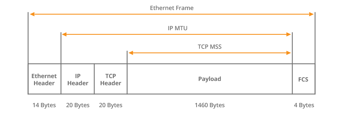 Picture 1 – TCP MSS 1460 Bytes Inside Ethernet Frame
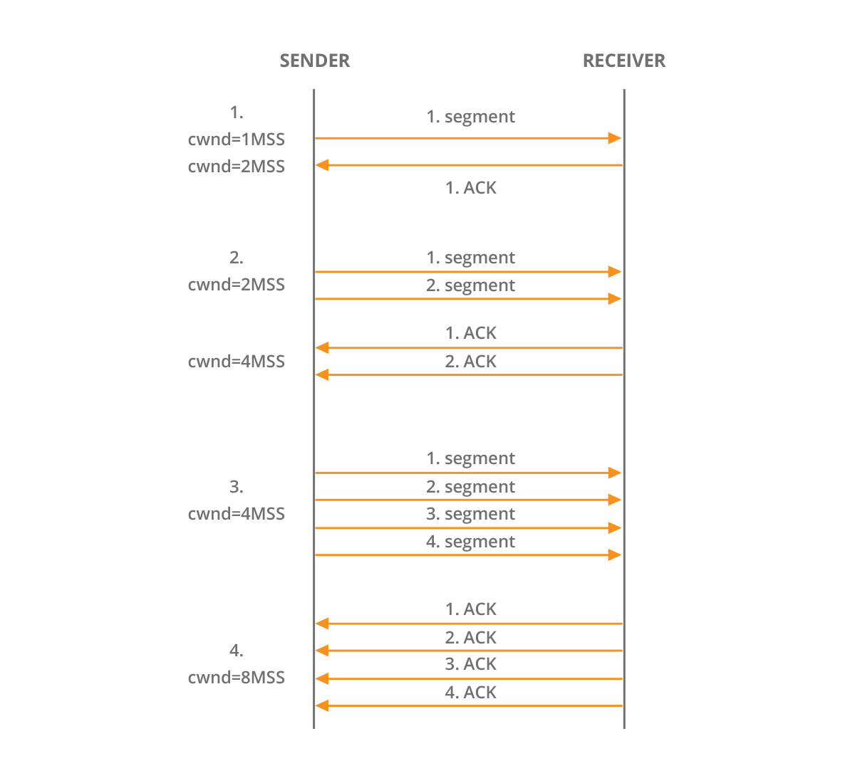 Picture 2 – Old Tahoe Slow Start Algorithm
When the slow start threshold (ssthresh) is reached, TCP switches from the slow start phase to the congestion avoidance phase. The cwnd is changed according to the formula: cwnd = cwnd + MSS /cwnd after each received ACK packet. It ensures that the cwnd growth is linear, thus increased slower than during the slow start phase. However, when TCP sender detects packet loss (receipt of duplicate ACKs or the retransmission timeout when ACK is not received), cwnd is decreased to one MSS. Slow start threshold is then set to half of the current cwnd size and TCP resumes the slow start phase.
The TCP Tahoe has been in use for many years, however there are some modern TCP variants such as TCP CUBIC that are better suited for transmission over the long fat networks (LFN). Those are the high-speed networks with high round trip time (RTT). The benefit of using the CUBIC variant is that the update of the congestion window is not dependent on the receipt of the ACK messages, thus is independent from the high RTT in LFNs. Instead, window growth depends only on the real time between the two consecutive congestion events. The growth of TCP CUBIC is CUBIC function using both concave and convex profiles after the last congestion event.
| Note: RTT is measured with ping command. |
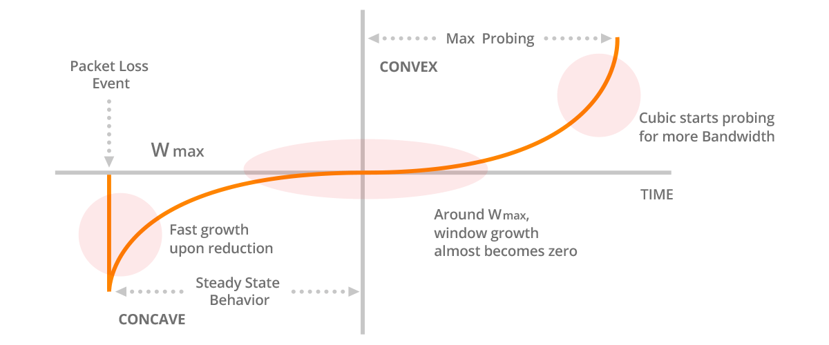
Picture 3 – Window is CUBIC Function with Concave and Convex Profiles
Just before the most recent loss event, CUBIC registers the congestion maximum window size (Wmax). After the loss event, the congestion window is reduced. Initially, the window size grows very fast in a concave region of the CUBIC function, however as it gets closer to Wmax value, the growth slows down. At the time it reaches Wmax, the gain is almost zero. In the convex profile of the CUBIC function, the window growth is initially slow. The time spent between the concave and the convex regions allows the network to stabilize since the cwnd is not rapidly increased under the high network utilization. As cwnd moves away from the Wmax value, the window growth gets faster, so the capacity of the high speed links can be utilized more effectively.
CUBIC has been used in Linux since the kernel 2.6.19 version, replacing its predecessor BIC-TCP. Since then it has been actively tested and used in many deployments. It proves itself to be well suited for transmission over the long fat networks with both high capacity and RTT. In the future it may be replaced by the Bottleneck Bandwidth and RTT (BBR) congestion control algorithm developed by Google. BBR uses a different approach to control congestion, the one that is not based on packet loss. BBR measures the network delivery rate and RTT after each ACK, building an explicit network model that includes the maximum bandwidth and the minimum RTT. Based on the model, BBR knows how fast to send data and the amount of data it can send over a link. BBR has significantly increased throughput and reduced latency for connections on Google’s internal backbone networks, google.com and the YouTube Web servers [1]. According to Google’s tests, BBR’s throughput can be as much as 2,700x higher than today’s best loss-based congestion control mechanisms while the queuing delays can be 25x lower [2].